
A few weeks back, a prominent person in the audio community shared with me their opinion that DSD is a different thing entirely from PCM, and was surprised to hear me insist otherwise. On the face of it, of course, they are indeed very different formats. PCM maps out the actual amplitude of the original waveform, sample by sample. DSD, on the other hand, looks like a completely different animal, and represents the waveform using a pulse-density modulation scheme, from which the original signal can be extracted by passing the digital bits themselves through a low-pass analog filter. For reasons that seem somewhat fuzzy to me, this is deemed to be inherently more akin to analog. Given that I’m a guy whose turntable still sits atop his audio stack, why would I bother to take issue with that?
For most practical purposes, the whole subject is an academic argument over little more than semantics. But DSD does have some very fundamental differences in its digital nature when compared to PCM. For example, you can’t mix multiple tracks together in DSD…or blend a stereo feed into a single mono channel. You can’t do EQ. You can’t even do something as rudimentary as volume control.
The big issue with DSD, and the reason for all these limitations, is that unlike with PCM, the signal itself cannot be extracted simply by examining the bitstream. Most people are apparently comfortable with the familiar arm-waving explanations for how a signal is represented within a DSD bitstream as a pulse-density-modulation scheme, but while that is indeed a valid characterization, it does little – nothing, actually – to help you understand how the signal is actually encoded within the bitstream. For example, on what basis would you determine what resolution it has – is it better or worse than CD? How low is the noise floor – is it better than 24-bit PCM?? What is the bandwidth – does it go above 50 kHz? In any PCM format, these questions are unambiguously answered. But not in DSD. Where exactly in that 1-bit stream can I find my high-resolution audio data? I thought it might be instructive if I were to return briefly to Copper and set about exploring this issue, and hopefully frame it in terms everybody can understand…or maybe at least follow.
PCM is based on the well-known sampling theory of Claude Shannon. Provided an analog signal includes no frequency components above a certain maximum frequency, then that analog signal can be losslessly represented in its entirety by discretely sampling it using a clock with a sample rate no less than twice the maximum frequency present within the signal. The italicized qualifier “in its entirety” is important here, because Shannon’s theory informs us that the totality of the sampled data enables the entirety of the original signal to be faultlessly reconstructed, even at arbitrary points in time that lie in between consecutive sampled values.
Let me start with a simple analog signal, a sine wave. In the diagram below, a sine wave with an amplitude of ±0.6 is shown. The red dots indicate the points at which the waveform is sampled. It represents an ideal situation in which the waveform is perfectly sampled:

In the next diagram, however, I introduce a crude sampling constraint. I require the samples to be evaluated to the nearest multiple of 0.2 (corresponding to a bit depth of approximately 4 bits), chosen for clarity’s sake so we can clearly observe the consequences. Here we can see that this results in a type of error known as a quantization error. In effect, the sampled signal is the sum of two signals, the original intact waveform (in blue), and the sampled waveform corresponding to the quantization error (in black).

This is PCM in its simplest form. It is an accurate representation of the original waveform, only to the extent that the waveform corresponding to the quantization error is inaudible. If it is in fact inaudible, then you will have succeeded in recreating the original waveform.
It must be noted, however, that the question of the audibility of the quantization error waveform is not as straightforward as you might imagine. At first glance it looks like random noise, and indeed if it were random noise we would be completely justified in treating it as inaudible, provided that it was at a sufficiently low level. But if components of the quantization error signal were correlated with the original waveform, their audibility can be quite significant, even at surprisingly low levels. Correlated signals fall into the broad category of “distortion,” which is a well-known and complicated topic. Some forms of distortion are known to be less pleasant on the ear, and significantly less tolerable than others. So it would be good if we could eliminate from the quantization error any remnants of correlated signals, and leave behind only pure random noise. It turns out that we can easily do exactly that, using a process called dithering, which I have covered previously, way back in Copper Issue 6.
That, in summary, is pure PCM. We can use it to accurately encode a mixture of the original analog signal, plus a sprinkling of added noise. And by using 24-bit encoding, that sprinkling can be waaaaay down below the residual noise floor of any analog signal that you might have available as your source.
Back to our little diagram, then. We can interpret the exact same picture in a slightly different way. We could interpret it as saying that by adding a very particular noise waveform to our original waveform, we made the amplitude of the resulting waveform correspond exactly to the nearest available quantization level at every single sampling point. In other words, we can argue that we effectively eliminated all quantization errors entirely, by the simple act of mixing in a special noise waveform of our own making.
At this point, I would really like you to go back and read the previous paragraph again. Keep reading it until you absolutely get it. It is key to what comes next.
OK, let’s move on. We’ve just established that an ideal PCM signal comprises the original audio signal, plus some added noise. We’re talking about the entirety of the original audio signal, in its pure unadulterated form. Not a 16-bit version of it, not a 24-bit version of it, but the entire, clean, original waveform in all its glory. The 16-bit (or 24-bit) version is what we get AFTER we’ve added in the noise, and stored the result in a 16-bit (or 24-bit) word.
We would find ourselves living in a perfect world if we could then just extract that added noise, because if we could, we would be left with only the pure, original, audio waveform. Unfortunately, that’s just not possible. The problem is that the noise, as described, occupies the exact same frequency space as the signal. Such noise cannot be extracted from a signal – that is the very nature of noise itself. The only practical way of separating out noise is to filter it out, and it doesn’t help all that much if we end up filtering out parts of the signal at the same time.
Let’s return to our little diagram, and this time take the same concept to its extreme. In the version below we have allowed only two quantization levels, at +1 and -1, and consequently the noise signal itself has become huge. The diagram, unfortunately, may be difficult to interpret, and will require some concentration on your part. The blue line and the red dots are the original waveform as before, and the black lines are the added noise samples. The green dots represent the sum of the waveform plus the added noise. The green dots, as you can see, occupy only the positions +1 and -1.

You can clearly see that the added noise is of a much higher magnitude than was the case previously. In fact, the noise itself has peaks that are comfortably higher than ±1. [Note: For what it’s worth, although this noise signal does in fact encode a noise waveform, the noise waveform in itself is completely irrelevant – it is only the specific values at the sampling points that have any relevance at all.] Now, this serves to prompt a big question – “So what?” Because, if the noise is truly massive, and we can’t separate it from the signal, have we accomplished anything?
But first, we need to make a quick detour on the subject of implied precision. If I were to propose that you phone me at one o’clock, in your mind there will be some approximation as to how precise that appointment is meant to be. You might, for example, assume that five minutes before one, or five minutes after one, would be acceptable. But if I instructed you to phone me at 1:13:22 – that is, 13 minutes and 22 seconds after one pm, you may get a different impression of just how precisely I wished for our appointment to be. In other words, the precision with which a number is stipulated is often presumed to convey something about the precision of the quantity which the number represents. Therefore, the number “1” is taken to mean, “roughly, approximately, 1.” Whereas, in comparison, the number “1.000000” would be taken to mean exactly 1, with a precision of at least 6 decimal places. In the following paragraphs I have therefore chosen to write the numbers +1 and –1 as +1.00000[…] and –1.00000[…] respectively, to indicate that I am stipulating numbers with an extreme precision of many decimal places, that “+1” and “–1” might not otherwise convey.
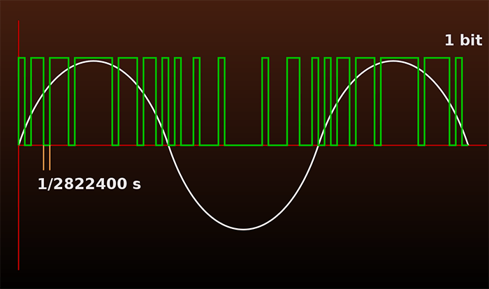
Back to our “So what?” question. It turns out that we do in fact have a route forward. Since the addition of the signal plus the noise always comes to either +1.00000[…] or –1.00000[…] at the sampling points, all we need to represent the result of the addition is a 1-bit number. A +1.00000[…] result is represented using “1” and a –1.00000[…] result is represented using “0.” Compared to 24-bit PCM, we would only need 1/24th the amount of file space to store the data. Perhaps that could open the door to a practical solution. If, for example, we were to increase the sampling rate by a factor of 24, we’d end up with a file of the same size as the original, and maybe we could take advantage of that in some way. For example, by way of illustration, let’s consider a 24-bit 88.2kHz high-resolution PCM file. If we were to reduce the bit depth to 1-bit by adding some of that “magic noise,” and increase the sample rate by a factor of 24X to 2.114 MHz, we will end up with a 1-bit file the same size as the original 24-bit file. Can we do something useful with that?
The thing about a PCM file with a 2.114 MHz sample rate is that, according to the Nyquist criterion, it can encode signals with a bandwidth of up to 1.057 MHz. But we only need 20 kHz (let’s be all high-end-y and call it 30 kHz) to encode all of the audio frequencies. That means there is a region from 30 kHz all the way to 1.057 MHz that contains no useful audio frequencies at all. Let me write that another way at the risk of belaboring the point. The region of 0.030–1.057 MHz contains no audio data. All the audio data lives below 0.030 MHz. That’s a tiny corner of the overall addressable frequency space.
Time to go back to the last diagram and take a closer look at it. All those black lines represent added noise. Each line can take on one of two possible values. Either it can be a positive number, the exact amount needed to raise the amplitude to +1.00000[…], or it can be a negative number, the exact amount needed to reduce the amplitude to –1.00000[…]. The important thing to note is that, conceptually at least, it really doesn’t matter much to us either way.
Given that every second of music will require 2.114 million of these noise samples, and that each and every one of them can assume one of two possible values, there are an almost uncountable number of permutations available as to how we could arrange those noise samples across the entirety of an audio file. The question is, can some of those permutations possibly turn out to be useful?
Recall that the only way to separate noise from a signal is to filter it out. Suppose we were to arrange the noise so that it only occupied those frequencies above 0.03 MHz. If we could do that, then all we’d need to do is pass the signal through a low-pass filter with a cutoff of 30 kHz. All the noise would then be stripped off, and we’d be left with the original unadulterated audio signal. This would be a very workable solution indeed … if we could figure out a way to actually do it.
That way is called sigma-delta modulation, (or, delta-sigma modulation), but this is not the place for me to describe how it works. You’ll just have to take my word for it that it does. A sigma-delta modulator does just what we want here. It creates the exact kind of noise signal that we are looking for through a process called noise shaping. It creates a “magic” noise signal that raises or depresses every sample value to +1.00000[…] or –1.00000[…], while keeping virtually the entire spectrum of the noise carefully above the audio bandwidth, where it can be easily filtered out.
There are theories that analyze and quantify just how much of this noise it is possible to push up into the unused high frequencies. The basic noise shaping theory was developed by Gerzon and Craven, and we don’t need to go into it here, but it essentially quantifies the “no free lunch” aspects of the process, and provides fundamental limits beyond which the magic cannot be pushed. I don’t have space to dig into it here, but let’s be clear, those limits do not prevent us from achieving the kind of audiophile-grade performance we desire. Far from it.
The main finding from Gerzon and Craven is that we need to push the sample rate out to quite high levels. It turns out that our simple solution of pushing it out by a factor of 24 in order to keep the same file size is not really far enough. Actual DSD (Direct Stream Digital) runs at a sample rate of 64 times 44.1kHz (which comes to 2.82 MHz), and in practice that represents the lowest sample rate at which adequate performance can be achieved. Today, it is commonplace to refer to that as DSD64. By doubling the sample rate to 128 times 44.1 kHz we get DSD128, and that arguably represents the sweet spot for the technology. But DSD256 is now being used in serious high-end studio applications. There are even people who are playing around with DSD512. At these colossal sample rates, at least from a theoretical perspective, any additional benefits start to become increasingly marginal, and the file sizes needed to store them can start to become pretty unwieldy.
So there we are. DSD, at its core, is simply a way of representing PCM audio data. The actual audio signal itself is a PCM-encoded audio signal that has been subsumed within an avalanche of high-frequency noise, such that the only way of extracting it is to filter out that noise. The achievable resolution is determined by just how much of the “magic noise” signal still resides within the audio band, and current SDM technology places that at about –120 dB or thereabouts, corresponding to ~20-bits of PCM resolution. The achievable bandwidth is determined by the sample rate, and DSD64 can achieve something close to 30 kHz (depending on how you choose to define it). That the ‘magic noise’ can be filtered out as effectively in the analog domain as in the digital domain has opened the door to a class of DAC designs which today totally dominate the DAC market.
There are those who insist that DSD sounds better than PCM, but that’s not an argument that makes any sense to me. DSD and PCM don’t have “sounds” per se. The things that DO have “sounds” are the processes that encode a signal into PCM and/or DSD, and that decode them back into analog, because these processes are generally not lossless, and that’s a separate discussion entirely. By contrast, BY FAR the biggest contributors to sound quality are the original recording engineers, and the lengths they are willing to go to in order to achieve the best sound possible. For these people, recording in DSD forces them to abandon all of the über-convenient post-processing digital chicanery available at the click of a ProTools mouse. Maybe – just maybe – that’s the most important observation of all.
Header image courtesy of Wikimedia Commons/Pawel Zdziarski, cropped to fit format.
