


As most audiophiles and readers of this magazine are aware, the subject of audio cables can be fraught with opinions, information, misinformation, heated discussions on forums and more. From time to time, Copper has run articles about cables and will continue to do so. In Issues 48, 49 and 50, Galen Gareis of ICONOCLAST cables and Belden Inc., and Gautam Raja wrote a series of articles on the importance of time-domain behavior and how it affects the sound and performance of audio cables. In this series, Galen expands upon the subject and takes a deep dive into a critical but not often discussed aspect of cable design: the velocity of propagation (Vp) of audio signals.
Introduction
Audio speaker and interconnect (IC) cables all have an Achilles’ heel that must be directly addressed. However, it is often completely ignored.
The performance of audio cables is more about the time-domain dependency of the signal through the audio band than on the factors of simple attenuation, resistance, or the concept that we just need to achieve low resistance, capacitance and inductance to design a good cable.
Also, while it might seem theoretically ideal, we can’t allow cable capacitance or inductance to simply go “as low as we can design it” without balancing the cable’s non-linear velocity of propagation through the audio frequency range.
The key concept here is that the velocity of propagation (Vp) is different for different frequencies in the audio range, and this will affect cable performance.
For example, if the upper-midrange and high frequencies arrive at the speaker (and your ears) faster than the lower frequencies, the timing of the music will literally be off, as well as the relationship between the fundamental frequencies and the overtones. The cable may sound too bright or too dull.
What changes are happening when we consider the velocity of propagation differential and what can we do to take it into account in our designing a cable? Each frequency will arrive at a different time at the end of the cable. Harmonics are tightly connected to the fundamental tone, and time based distortion of a sufficient magnitude will alter how we hear musical tones, a tone being a fundamental plus the harmonics.
Fundamental Factors In Cable Behavior
The math behind the non-linearity of the velocity of propagation isn’t new. In fact, Belden explored the issue as far back as 1974 and 1984 in their in-house publication Belden Innovators SPRING magazine articles (available upon request). However, in practice what we need to know and to measure is seldom used to fully optimize an audio cable’s performance. Two cables with the exact same bulk resistance, inductance and capacitance (R, L and C) can sound decidedly different based on the Vp management used in their designs.
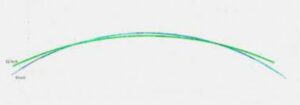
The graphs below are for a specific cable resistance, inductance and capacitance (R, L and C). The fundamental shape and curve of the traces are universal for low frequency cables that handle the audio band which is electrically low in frequency. The exact values along both traces will vary based on a cable’s particular design parameters, but all low audio and low frequency cables are affected in the same manner by how the physics shapes the general data.
The plots show the cable’s Velocity Factor (Vp) percent and Impedance (Zo). (The two papers from which these graphs are derived are also available.)
Notice that the two sets of fundamental traces, from two independent sources, are the same. The top set is calculated and the bottom set is empirically measured cable data. No matter what passive cable we test through the low frequencies, the shape of the curves will be a like pattern.
http://web.mst.edu/~kosbar/ee3430/ff/transmissionlines/z0/index.html (The link has expired; I have the paper.)

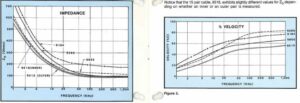
The above two separate sources for velocity non-linearity show the exact same cable properties for impedance at low frequencies. Impedance goes up, considerably, as Vp goes down.
You can’t escape Vp non-linearity through the audio band and the rise in impedance it causes. Physics isn’t on our side.
Another point to consider is that an audio cable isn’t a transmission line, which is a cable designed to carry and accommodate electromagnetic (EM) waves in a contained manner. These cables operate over large electrical distances with minimum losses and distortion.
At audio frequencies the wavelengths are too long and won’t “fit” inside a cable’s length. Even if we wanted to accommodate just one full wave period, the wavelength is too long in the low-frequency range we call audio. For example, in free space a 20 kHz wavelength is 14,989 meters long;
λ = C/f
Where,
λ (Lambda) = Wavelength in meters
c = speed of light (299,792,458 m/s)
f = Frequency
In an audio cable it is fore-shortened by the Vp of the dielectric which is around 50% at 20 kHz, but we are still looking at a long wavelength; 7,494.8 meters or 24,588 feet.
λ = (0.5)*( 299,792,458 m/s)/ 20,000 Hz = 7,494.8 meters
Ideally, we need a cable of at least ten wavelengths to reach a stable TEM (transverse electromagnetic wave) situation. In a true TEM wave, the signal is trapped between the inner surface of the shield and outer surface of the center conductor and inside the dielectric in a coaxial cable. In a twisted pair it is trapped between the inner surface of the two wires and also in the dielectric. Since a twisted pair has a higher loop DCR (Direct Current Resistance) component than a coaxial cable with a like-sized center wire, the twisted pair attenuation is higher. Twisted pair noise immunity can be improved in a true balanced circuit using CMRR, Common Mode Rejection Ratio, a configuration where the noise is subtracted out from the signal. What is common to both wires is the noise, hence the term CMRR.
However, I will never adhere to the supposition that we have true TEM function-type reflections in audio cable, unlike where impedance is matched to a load, like an RF cable. Impedance isn’t and can’t be matched in the audio frequency range and we’ll see why in this series. (We’ll also see why RF cables aren’t ideally matched, either, even at the exact same value as a load resistor.)
In order to understand what’s happening in audio cable we need to understand why RF cable has some decided advantages over audio when it comes to system matching (in RF applications). The velocity, or speed, of the TEM wave trapped inside the wire either between two wires (twisted pair), or between a wire and a shield (coaxial cable) is a constant at RF. It does not fundamentally change with frequency. I say “fundamentally” because some will say if it changes any amount at all it “matters.” (OK, I’ll give the perfectionists among you +/- a few percent.)
There are several methods to calculate or measure RF impedance. Don’t try any of this at audio frequencies or even below 1 MHz. 1 MHz isn’t truly reaching the impedance asymptotic stability level.
The following method is known as the ratio method. Here we can look at a known cable’s impedance that we feel is accurately reported under test correctly. We can take the ratio of the center wire diameter to inner shield diameter (the dielectric’s diameter), and use that to design a cable with a larger diameter or even determine what its impedance will be when compared to known ratios. This works for twisted pairs, too, since we look at each insulated wire as a coaxial cable, but with both placed two in parallel. For example, two 50-ohm coaxial lines in parallel double the center to center distance so we have less capacitance and a higher 100-ohm impedance, for instance.
We need to make sure that the dielectric velocity of propagation is the same, however, or this won’t work. The speed of the electromagnetic wave is also changing the impedance of the cable in the calculations and ratio measurement.
Example:
| 9110 RG59 75-ohm | 9118 RG6 75-ohms | |
| CENTER WIRE | 0.032 20 AWG | 0.040” 18 AWG |
| DIELECTRIC OD | 0.144″ | 0.180″ |
| Vp | 83% | 83% |
| RATIO | 4.5 | 4.5 |
If I match the ratios and dielectric materials I will have the same impedance as the reference ratio. Pretty easy if the reference cable is made right and to the value you want.
1.0) We can calculate the impedance with several equations, the easiest uses the resonance method. This measures capacitance at 1 KHz, and then using two RF frequencies uses a resonance property to calculate the velocity of the signal in the cable at RF. Now we have nothing but C and Vp. That’s all we need;
101670/(C*V) = impedance at RF. This equation is from MIL-C-17G section 4.8.7.2.
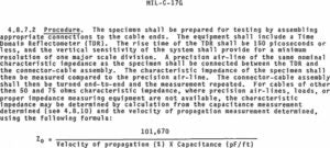
What is important is the relationship between velocity of propagation at a specific impedance and the capacitance in the RF range. We can’t use this relationship in the audio frequency range as Vp is non-linear.
2.0) A measurement, not calculation, can use a variable resistive bridge to measure a cable into a load that is resistive and can be varied, to determine the impedance. This relies on the cable’s structural return loss or SRL.
SRL is the signal return loss of a cable relative to its own impedance, caused by manufacturing imperfections in a cable.
How do we determine the impedance is the “structure” of the wire? In the test the load is varied until we measure a minimum reflection of the test load swept across an RF band. The resulting fitted impedance graph is the cable’s natural impedance, but only at RF, where a true transmission line’s property exists.
3.0 ) There is also return loss, or RL, which is a stricter criterion than SRL. Here is the difference between the two;
- Structural return loss defines how precisely we manufacture a cable, and therefore how uniform the impedance is at that cable size.
- Return loss defines whether we made the cable the right size to achieve the desired fixed load impedance.
RF cable is mostly resistive, so we can use a resistive load. The cable, however is not a pure resistor even at RF. What does this do? Is it similar to an audio cable’s changing impedance with frequency?
Here is what happens in an RF twisted pair, which has enough geometric deviation to “see” electrically relative to a coaxial cable’s geometric perfection in terms of much more consistent electrical behavior. The twisted pair’s higher geometric variation is handy since it is allows us to show the effect of measured electrical RL performance with a graph. On the left side of the graph is impedance. This cable is supposed to be 100-ohms swept, or tested using a frequency sweep from 1-100 MHz.
If we sweep to test the return loss, RL differs from SRL as the load is fixed at 100-ohms. Since we can’t cheat and adjust the load to minimize reflections, we get a bunch of RL points in dB, I plotted in the X-axis with the impedance of that point in the Y-axis.
-What’s weird about this graph?
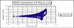
Let’s just look at the 100-ohm center frequency. We see that RL varies from –55 dB (smaller is better) to –25 dB. How is this happening at exactly a 100-ohms impedance? It’s because the impedance is a vector sum of the cable’s real (resistive) and imaginary (capacitance or inductance, but usually capacitance) vector magnitudes.
The vector is 100-ohms but it isn’t resistive anymore so we get reflections. The size or length of the resistive vector missed true 100-ohm values.

This idea tends to escape peoples’ interpretation of RF impedance. What about the points above and below the 100-ohms reference? Here is where people seem to go; we have impedance values higher and lower than a 100-ohm cable. But, some impedance values that miss the 100-ohms center frequency have lower RL than those on the 100-ohms line! The 100-ohms RL line stops at ~ -28dB. We can see several data points that are not 100-ohms, as high as 115-ohms and as low as 90 ohms, that are better than –28 dB RL value. It all relates back to the real versus imaginary component of that specific impedance vector.
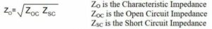
But, impedance at RF is still not an easy matter to define, as it relates to signal transfer with all else this going on. In this next example we’ll use an open-short-load and open-short impedance test.
Let’s take a pause here and ask: is audio cable “related” to RF cable? We see reflections in an audio speaker cable off a much more reactive load than RF cable so the expected energy transfer is far harder to predict.
This next example tries to move the testing to low frequency audio cables even if we can’t accommodate the wavelength as a transverse electromagnetic wave.
4.0) This method is most common for very low frequency tests. The impedance is calculated from the open and short measurements (see the chart). This method de-imbeds, or removes, the “load” and concentrates on just the cable itself. It also is better the longer the cable can be for lower frequencies. As was mentioned earlier, an audio cable can’t be too long if we want to test impedance! We would, of course, never ever use one that long and that’s part of the problem. The data provides the signal magnitude and phase.

From the chart shown above, we see that impedance drops as we increase the frequency until it begins to flatten to ~60-ohms at about 1 MHz. Why?
But first, we need to emphasize a fundamental concept relevant to cable testing and design;
The math fits the physics, not the other way around.
Physics limits what we can do, and how we derive equations to fit nature to printed paper. Therefore, our model equations are often not perfectly correct along every point within a curve. This is called “curve fitting”. In the case of some math the results are called models because they are close to the real thing, but they aren’t completely accurate. Here’s an example:
A tonearm tracking curve is only correct in specific spots. The correct tracking geometry is not really “exactly” along the entire curve. A longer tonearm will improve how close we are to “right” so we can alter the design to reach different compromises.
The model suggests we are correct in exactly two spots, seen in the graphs of two tonearms of different lengths. One is a better model to theoretical ideal but both are exactly right at just only two spots. (Factor in overhang errors, stylus alignment and other issues and it becomes apparent the we need to consider what is happening in realty as well as mathematical models.)
This is only one example of why we can’t rely on mathematics – we can use it as a guide, but have to do the measurements to verify what’s happening in the real world. There are always variables that can’t be easily and correctly assessed using equations in the process of getting a model to be as accurate as we may need. Engineers characterize accuracy estimates as orders of approximations – zeroth-order, first-order and so on. It results in equations getting more complex as we add error correction.
Eventually an equation is accurate enough, and verified to real measurements, to become useful in designing a cable (or product).
Back to our analysis of the velocity of propagation and its importance in cable design: We can look at a few examples and see the actual Vp responses of known cables against measurements that the equation(s) are modeled from and see how they compare.
 The above graphs show the Vp response of several audio cables. The equation derived from the curves is;
 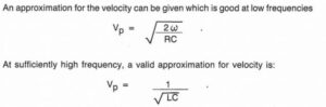 If we graph a cable, in this example a Belden 9515 multi-pair cable, and apply the low-frequency approximation equation, we see the data table below. The Vp values across frequency closely match the plotted swept data from our measurements. In this Vp example the impedance rises as frequency drops. (If R (resistance) or “C (capacitance) gets too high, we need to redefine the equation.)
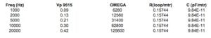
We can see that in the low frequencies, we need a different equation to account for specific variables going to “zero” (as low as a variable will go) or “one” (as high as a variable will go) as we increase the frequency into the RF band. At RF frequencies we can use a single Vp value above 1 MHz. However, this has to be abandoned at audio frequencies. We’ve seen this earlier in the article in the measure of impedance, and since Vp is part of the impedance equation, since it determines capacitance, this isn’t a surprise after all. If we hold the impedance and change either C or Vp variable, the opposite one has to change; Zo= (101670/C*Vp).
In the example below, we have three equations for approximating cable impedance measurements. Notice that the curve rises as we drop in frequency, and is orders of magnitude higher than at RF. This is why we can’t make a “flat” or low-impedance cable through the audio band. (At RF, impedance is essentially resistive).
 We also have simpler approximations we can use at low and high frequencies starting at 100 Hz (for low-frequencies) and at 1 kHz and 100 kHz (for higher frequencies). G, the mathematical symbol for conductance, is the reciprocal of resistance in siemens (S) or mhos units. L and C are in farads and Henrys. Yes, you need all the zeros; 12 pF is 0.000000000012 farads.

These simple equations don’t have “frequency” in the equation at the very high frequency ranges, so their results produce straight line graphs. For RF that’s all we need, though. The mid-range impedance equation does have frequency, OMEGA (v), which is (2f). R and C is length dependent so we have to set a length (SI units for instance). We also see the transition equation is a curved fitted line.
The “easy” definition of low-frequency impedance ignores reactive (capacitive or inductive) effects at the very low-end and sees impedance as just DCR, Direct Current Resistance. Reactive effects are worse as we drop in frequency, so it involves a lot more complicated approximation and doesn’t allow us to just ignore reactive effects from capacitance and inductance at low-frequencies.
At RF we can ignore reactive effects, and our earlier twisted pair impedance plot reactive RL measurements show that the vector magnitudes are close to a resistive value at the target impedance. We have no load reflections or out of phase information to worry about if the cable has good RL (low reflection) attributes.
The input impedance of a transmission line, open at the far end, looks like a capacitor. The reactance is worse at lower frequencies because capacitors pass higher frequencies better than lower frequencies. Impedance at low frequencies starts very high and drops very low as frequency goes up. Capacitors pass AC signals better the higher we go in frequency. Higher frequencies have lower Xc, or resistance to signal flow.
We see the higher impedance values at the low-frequency end, and dropping impedance values at the high frequency end caused by Vp and capacitive reactance change. The reactive effects slowly diminish at higher frequency (don’t impede AC current flow). The RF Vp reaches a steady state based on the dielectric. Vp is purely based on the material property of the dielectric at RF; 1/ SQRT(dielectric constant).
In the next installment, we’ll look at practical ways to change the velocity of propagation and improve signal linearity, among other subjects.
0 comments