Another common usage of the term “linearity” in electronics refers to linearity in amplification at different levels; this can be called “dynamic linearity.”
As an example, let us take an imaginary amplifier, which is meant to have an amplification factor of 10. This means that if we feed a 1 kHz sine wave having an amplitude of 1 volt RMS at its input, we shall expect to see a 1 kHz sine wave having an amplitude of 10 volts RMS at its output, without any additional elements.
Before going further, let’s review frequency and phase linearity, which we covered in Part One. Frequency linearity in the 20 Hz – 20 kHz bandwidth would mean that if we feed any frequency from 20 Hz to 20 kHz at 1 volt RMS to the input of our amplifier, we shall see that same frequency at 10 volts RMS at the output. Phase linearity in the 20 Hz – 20 kHz range would require that the phase of a sine wave at any frequency from 20 Hz to 20 kHz would be exactly the same at the output, as it was at the input. (This would imply a linear frequency response over a much wider range than the specified 20 Hz – 20 kHz.)
So, frequency linearity looks at the relative amplitude of different frequencies. Phase linearity looks at the relative phase between different frequencies.
Dynamic linearity investigates the linearity of the amplification process itself at different amplitudes (signal levels).
So, our theoretical amplifier will amplify 1 Vrms into 10 Vrms, 2 Vrms into 20 Vrms, 3 Vrms into 30 Vrms and so on. But can it be expected to continue this relationship between input and output, in a linear fashion, regardless of how high or low we go? If we feed 1,000 volts RMS to the input, will we get 10,000 volts RMS at the output?
The answer of course is no. Practical electronic circuits cannot remain linear indefinitely. There are limits imposed, both at high levels and at low levels.
Not only will we not get 10,000 Vrms for our 1,000 Vrms input, we also won’t be getting 0.000001 Vrms for our 0.0000001 Vrms!
All real-life electronic circuits have noise. This results in the ultimate limit for dynamic linearity capability at low levels. If the signal is lower than the noise floor of the amplifier, then it will remain buried in noise and there will not be any meaningful amplification. On top of this, various non-linear mechanisms in amplifier circuits may prevent linear amplification below a certain point. This would mean that if 1 Vrms becomes 10 Vrms, 0.1 Vrms may only become 0.9 Vrms instead of the expected 1 Vrms that the amplification factor of 10 would produce.
At high signal levels, there are power supply voltage, current and bias limitations. The amplifier can only supply so much voltage or current. So, while 1 Vrms becomes 10 Vrms and 3 Vrms becomes 30 Vrms, 4 Vrms may only become 32 Vrms, ruining the linear relationship.
A deviation from linearity is any change in the usual amplification factor of the circuit, at different amplitudes (signal levels). This usually results in distortion, which produces additional frequencies within the amplifier that are not present in the input. The type of distortion and the linear range of operation depend on the circuit design and amplification devices used.
We shall now leave our theoretical amplifier aside and see how dynamic linearity works in a real triode tube circuit. We will connect the cathode to ground and bias the grid at – 20 VDC to set the operating point. The audio signal fed to the grid will move upwards of – 20 VDC during the positive peaks of the wave and will move lower than – 20 VDC at the negative peaks. As we approach 0 VDC during the positive peaks, the grid starts to attract electrons and draws current. If the circuit supplying the grid with the audio signal cannot deliver this current, the positive peaks of the wave will be compressed and eventually chopped off! This reduces our amplification factor and results in second harmonic distortion (distortion that occurs at twice the fundamental frequency).

Average plate characteristics of an 845 triode from a 1933 RCA data sheet.
At the opposite extreme, as the grid voltage is lowered below – 20 VDC during the negative peaks of the audio signal, the electron flow is reduced. At a sufficiently negative grid potential, the current flow between anode and cathode is cut off. As the negative peaks of the audio signal approach this “cut-off region,” they are compressed and eventually chopped off. The amplification factor is reduced and second harmonic distortion is produced.
If the onset of grid current is at 0 VDC and cut-off is at – 40 VDC, then a symmetrical audio signal exceeding 40 volts peak to peak would reach both limits simultaneously. Both positive and negative peaks will be chopped off, resulting in third harmonic distortion, along with a reduction in the amplification factor.
But, even if we keep the input signal within the aforementioned grid bias limits, there are more creative ways to ruin linearity!
During the negative peaks of the audio signal, the current through the triode and its load is at a minimum, while during the positive peaks, it reaches its maximum.
A resistor is a fairly linear load, provided that the appropriate type of resistor is selected for its place in an audio circuit. However, resistors are wasteful of power and as such, their use is limited to small signal stages rather than power/output stages. At maximum current, the voltage drop across the resistor reaches a maximum and provided that the resistor is generously rated to not burn out from excessive power dissipation and that inductance/capacitance effects are not allowed to affect performance, the only major consideration in designing an audio circuit is if the power supply can actually supply the current being drawn, without an excessive voltage drop in the supply circuit itself! A voltage drop would compress the peaks of the wave, while a hard current limit would chop them off, again resulting in second harmonic distortion and a reduction in the amplification factor.
At minimum current, the voltage drop across the resistor is at a minimum and the peaks of the amplified signal can swing to nearly the supply voltage. This defines another hard limit, as any attempt to swing higher than the supply voltage will be simultaneously met by cut-off in the triode tube and the peaks will once again be chopped off.
Note that the power supply circuit is as important as the amplifier circuit topology and the amplification device itself in all of this, since all an amplifier does is modulate its DC supply voltage!
The quality, stability and linearity of the power supply at different frequencies and amplitudes of signal passing through the amplification device is what defines the ultimate performance capabilities of an amplifier.
While the resistor itself in theory, shouldn’t have any effect on this process, its resistance value will rise with rising temperature, and temperature will increase with rising current. A resistor will therefore produce thermal non-linearities through thermal modulation of its resistance value, particularly at very low frequencies.
However, at higher frequencies, the thermal inertia of the resistor will prevent “thermal tracking” of the signal waveform and will instead shift the value of resistance to a “thermal averaging” point.
Electromagnetic loads, such as transformers and inductors, are the norm for power/output stages. These are made by coiling wire around an iron core. They are some of the most useful components in audio but are extremely difficult to design, manufacture and implement, potentially opening up an impressive number of mechanisms for introducing non-linearities. Yet, if done right, they can sound fantastic and display enviable linearity.
The iron core can saturate at low frequencies, have losses at high frequencies, display magnetic hysteresis and its magnetic permeability can vary with the signal level and frequency. The coils have capacitance between adjacent turns and layers of wire, then there is leakage inductance on top, as well as wire resistance increasing with temperature.
The design of a high quality audio circuit is a delicate balancing act. What could improve performance in one aspect could degrade performance elsewhere, so everything needs to be taken into account at the same time. Electronics theory blends with mechanical engineering, particle physics, chemistry, thermodynamics, magnetism, acoustics, neurophysiology and psychology, requiring a multidisciplinary approach when designing audio equipment of the highest caliber.
It is part engineering, part art.
In the next episode, we will discuss linearity in more complex circuits, measurements and how it all relates to music.
Sidebar: Dynamic Linearity in Pictures
The following pictures are of oscilloscope traces (plotting amplitude against time) and spectrum analyzer traces (plotting amplitude against frequency) of a 1 kHz sine wave through a multiple-stage triode amplifier without feedback, using tubes of questionable linearity in a circuit intended to produce plenty of distortion for musical instrument amplification. It was chosen to clearly demonstrate the lack of dynamic linearity.

The scope trace (on the right) shows a sine wave, close to the limit of the linear region of the circuit. The analyzer trace (on the left) shows the fundamental at 1 kHz (to the left of the screen) and a second harmonic component at 2 kHz, around 30 dB below the fundamental (3% second harmonic distortion, 10 dB/div on the vertical scale).

As the amplitude of the 1 kHz sine wave is increased to exceed the linear region of operation of the amplifier, the scope trace shows a waveform with the negative peaks squashed, which is no longer symmetrical, due to the amplification not being linear. The analyzer trace displays the increase in the second harmonic distortion (the fundamental is displayed at the same level as before for an easy comparison), with the 2 kHz component now only about 14 dB below the fundamental (20% second harmonic distortion).

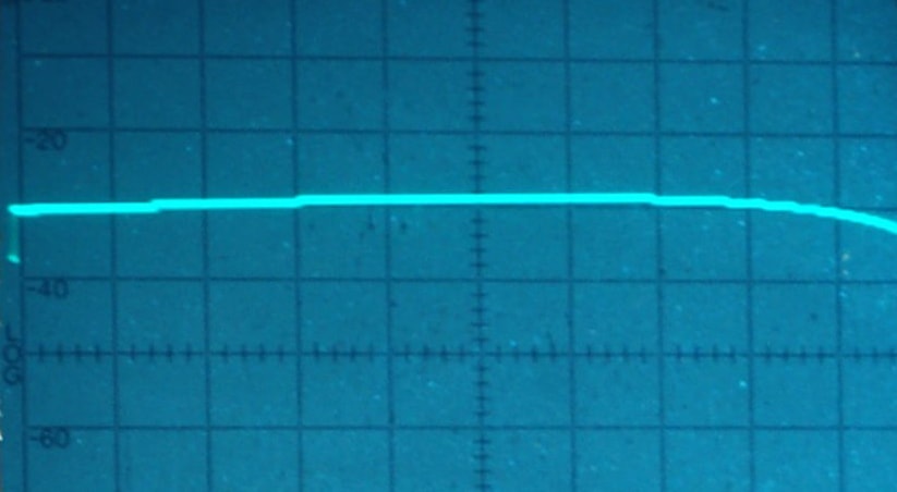
For clarity, traces with no signal input (the 1 kHz sine wave oscillator being turned off) are also shown. The scope trace is a straight line along the middle of the screen, representing the “zero” voltage line. The signal consists of positive peaks (rising above zero) and negative peaks (below zero). On the analyzer, however, the zero line is at the bottom of the screen. The sign denoting a positive or negative peak is discarded and we only see the absolute value of amplitude at each frequency. With no fundamental present at 1 kHz, there is also no distortion component at 2 kHz. An ideal, perfectly linear amplifier, would only show the fundamental component as presented at its input, with no additional components. In practice, even laboratory grade oscillators will have some residual distortion components.
All real-life devices and circuits produce distortion to some extent.